1.Bias and Variance
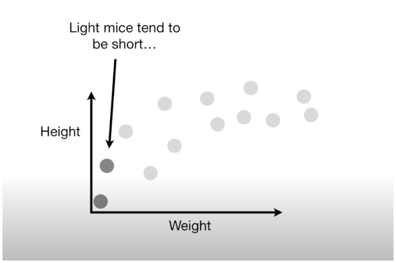
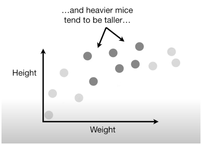
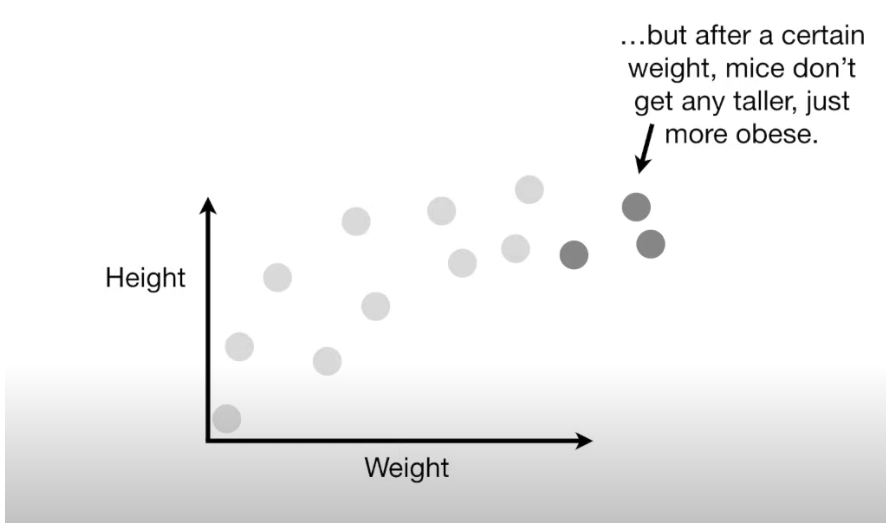
Imagine we have a set of data showing the weight and height of a bunch of mice. Generally, light mice are shorter, and heavier mice are taller, but after a certain point, as mice get heavier, they don't keep getting taller—they just become rounder. This curved relationship between weight and height isn’t perfectly predictable, so we’ll use machine learning to approximate it.
 |
 |
 |
|---|
Step 1: Splitting Data into Training and Testing Sets
When training a model, we don’t want it to learn from all the data at once because that doesn’t allow us to test its performance on new data. So, we split the data into:
! 400
- Training Set: This part of the data is used to “teach” the model.
- Testing Set: This is a smaller subset used to see if the model can predict new data points well.
In our example, we’ll use some mice’s weights and heights to train the model and hold back a few for testing.
Step 2: Trying Out Different Models – The Straight Line vs. the Squiggly Line
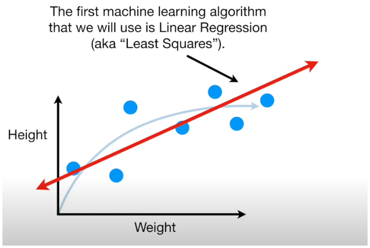
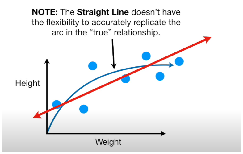
Imagine we start with linear regression, which fits a straight line to the data. This line is as close as possible to the points in the training set.
 |
 |
|---|
Here’s the catch: the actual relationship between weight and height is curved, and the line can’t capture it, no matter how hard we try. This introduces bias.
Bias is the error introduced by assuming a simple model (like a straight line) that doesn’t capture the data's complexity. In our case, the straight line has high bias because it’s too simple to match the curve.
! 300
To address this, we try a more flexible model—a squiggly line that can follow the curve closely, capturing the data’s details. This model has low bias since it more accurately reflects the data.
Step 3: High Bias vs. Low Bias
Now we have two models:
- Straight Line: Too simple and unable to follow the curve, resulting in high bias.
- Squiggly Line: Flexible and able to capture details, resulting in low bias.
Bias represents how consistently “off” a model’s predictions are due to oversimplifying the data. The straight line has high bias since it doesn’t adjust to the curve, while the squiggly line has almost no bias on the training set because it closely matches the data.
Step 4: Testing the Models and Introducing Variance
We test both models on the unseen testing set:
- The straight line performs consistently, showing low variance.
- The squiggly line fits training data very well but struggles with new data, showing high variance. It’s overfit to the training data.
Variance in machine learning is a measure of how much a model's predictions change with different data sets. High variance means the model fits the training data too closely (overfitting) and performs poorly on new data. Low variance indicates stability across data sets but may lead to oversimplification. The goal is to keep variance low enough for generalization but high enough to capture patterns.
The ideal model balances bias and variance:
- Low bias to capture real patterns.
- Low variance for consistent predictions.
We can reach this balance with techniques like regularization (simplifies complex models), bagging (uses multiple data subsets), and boosting (builds models sequentially to correct errors).
Recap: Why Bias and Variance Matter
Understanding bias and variance is crucial because it explains why some models work well on training data but fail on new data. If you can strike the right balance, you get a model that is both accurate and generalizes well, predicting new data with reasonable accuracy. That’s the essence of effective machine learning!